Inverse Wave Equation
Consider the 1d wave equation:
$$ \begin{equation} \frac{\partial^2u}{\partial t^2}=c^2\frac{\partial^2u}{\partial x^2}, \end{equation} $$ where $c>0$ is unknown and is to be estimated. A group of data pairs ${x_i, t_i, u_i}_{i=1,2,\cdot,N}$ is observed. Then the problem is formulated as:
$$ \min_{u,c} \sum_{i=1,2,\cdots,N} |u(x_i, t_i)-u_i|^2\ s.t. \frac{\partial^2u}{\partial t^2}=c^2\frac{\partial^2u}{\partial x^2} $$
In the context of PINN, $u$ is parameterized to $u_\theta$. The problem above is transformed to the discrete form:
$$ \min_{\theta,c} w_1\sum_{i=1,2,\cdots,N} |u_\theta(x_i, t_i)-u_i|^2 +w_2\sum_{i=1,2,\cdots,M}\left|\frac{\partial^2u_\theta(x_i,t_i)}{\partial t^2}-c^2\frac{\partial^2u_\theta(x_i,t_i)}{\partial x^2}\right|^2. $$
Importing External Data
We take the ground truth
$$ u=\sin x \cdot(\sin 1.54 t + \cos 1.54 t), $$ where $c=1.54$. The external data is generated by
    points = geo.sample_interior(density=20,
                                 bounds={x: (0, L)},
                                 param_ranges=time_range,
                                 low_discrepancy=True)
    points['u'] = np.sin(points['x']) * (np.sin(c * points['t']) + np.cos(c * points['t']))

    # Some data points are contaminated.
    points['u'][np.random.choice(len(points['u']), 10, replace=False)] = 3.
To use the external data as the data source, we define a data node to store the state:
@sc.datanode(name='wave_domain', loss_fn='L1')
class WaveExternal(sc.SampleDomain):
    def __init__(self):
        points = pd.read_csv('external_sample.csv')
        self.points = {col: points[col].to_numpy().reshape(-1, 1) for col in points.columns}
        self.constraints = {'u': self.points['u']}
        self.points.pop('u')

    def sampling(self, *args, **kwargs):
        points = self.points
        constraints = self.constraints
        return points, constraints
If large-scale external data are used, users can also implement the sampling() method to adapt to external data interfaces.
Define Unknown Parameters
IDRLnet defines a network node with a single parameter to represent the variable.
var_c = sc.get_net_node(inputs=('x',), outputs=('c',), arch=sc.Arch.single_var)
If bounds for variables are available, users can embed the bounds into the definition.
var_c = sc.get_net_node(inputs=('x',), outputs=('c',), arch=sc.Arch.bounded_single_var, lower_bound=1., upper_bound=3.0)
Loss Metrics
The final loss in each iteration is represented by
$$ loss = \sum_i^M \sigma_i \sum_j^{N_{i}} \lambda_{ij}\times\text{area}_{ij}\times\text{Loss}(y_j, y^{pred}j), $$ where $M$ domains are included, and the $i$-th domain has $N{i}$ sample points in it.
By default, The loss function is set to
square, and the alternative isL1. More types will be implemented later.$\text{area}_{ij}$ is the weight generated by geometric objects automatically.
$\sigma_i$ is the weight for the $i$-th domain loss, which is set to
1.by default.$\lambda_{ij}$ is the weight for each point.
For robust regression, the L1 loss is usually preferred over the square loss.
The conclusion might also hold for inverse PINN as shown:
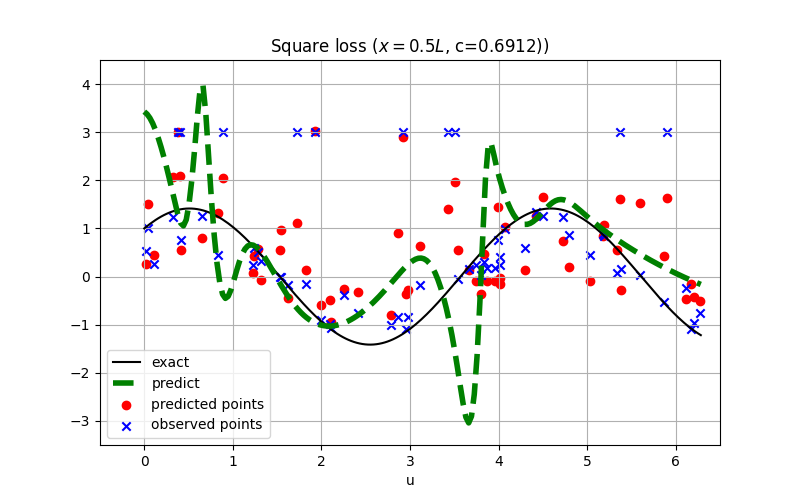
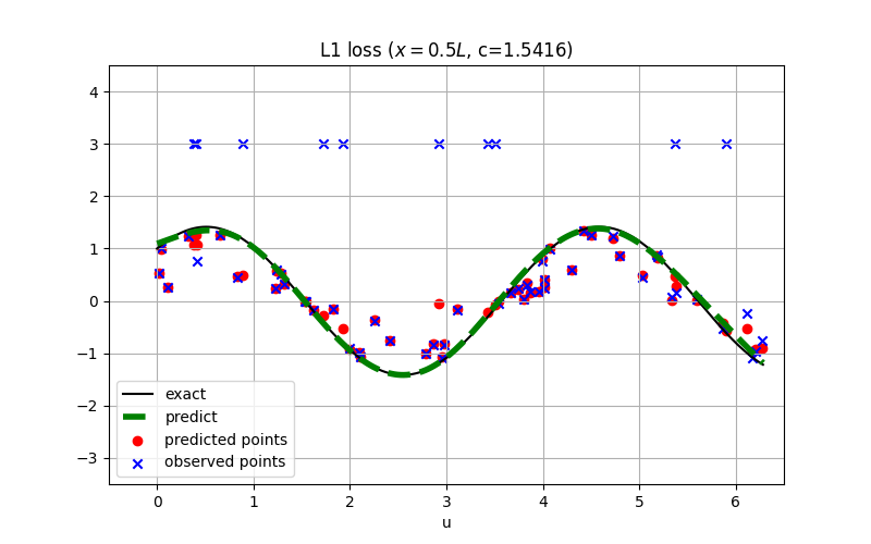
See examples/inverse_wave_equation.